

Bilinear Interpolation / Double Interpolation
How to use it
Review the methodology below to make sure it aligns with your project's requirements, then:
- Enter x1 and x2, the known bounding values for x, across the top, and x, the value you are interpolating for, between them.
- Enter y1 and y2, the known bounding values for y, down the side, and y between them.
- Enter P11, P12, P21 and P22, the known values at (x1,y1), (x1,y2), (x2,y1) and (x2,y2), in the corners.
- The interpolated value appears in the center of the grid, and updates as you type.
For interpolating between two points on a line, use the linear interpolation calculator.
Methodology, equations and example
This calculator returns an interpolated value using bilinear interpolation. "Bilinear" refers to a technique that uses the values at the four nearest data points to estimate the value at a point within the grid. The four points form a rectangle, and the interpolation is a weighted average of their values based on the distance of each from the point of interest. The technique is also called double interpolation, or bilinear filtering in some contexts.
The weights come from the distances between the point of interest and each of the four surrounding points: the closer a point is, the more it contributes. Each known value is multiplied by its weight, and the results are summed.
The method of bilinear, or double, interpolation:
Step 1: linear interpolation at point (x,y1): R(x,y1) = P11(x2−x)/(x2−x1) + P21(x−x1)/(x2−x1)
Step 2: linear interpolation at point (x,y2): R(x,y2) = P12(x2−x)/(x2−x1) + P22(x−x1)/(x2−x1)
Step 3: linear interpolation at point (x,y) using the results of Steps 1 and 2: R(x,y) = R(x,y1)(y2−y)/(y2−y1) + R(x,y2)(y−y1)/(y2−y1)
Step 4: substituting R(x,y1) and R(x,y2) gives the interpolated value at (x,y) as a single equation: R(x,y) = P11(x2−x)(y2−y)/((x2−x1)(y2−y1)) + P21(x−x1)(y2−y)/((x2−x1)(y2−y1)) + P12(x2−x)(y−y1)/((x2−x1)(y2−y1)) + P22(x−x1)(y−y1)/((x2−x1)(y2−y1))
The graph with the results above shows the four points and the point being interpolated.
Example
Calculate the total cooling capacity of a 5-ton Bryant® package unit from its performance data table, at design conditions of 79 °F condenser entering air and 65 °F evaporator entering wet bulb.
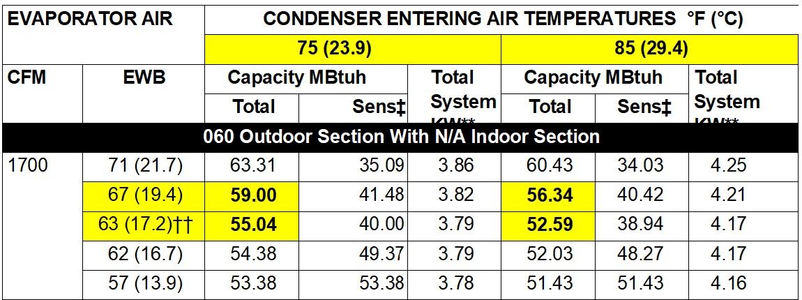
The example is solved two ways: first by three linear interpolations (Steps 1 to 3), then with the single bilinear equation (Step 4). From the table and the design conditions:
- P11 = 55.04 MBtuh, P12 = 59.00 MBtuh, P21 = 52.59 MBtuh, P22 = 56.34 MBtuh
- x1 = 75 °F, x2 = 85 °F, x = 79 °F
- y1 = 63 °F, y2 = 67 °F, y = 65 °F
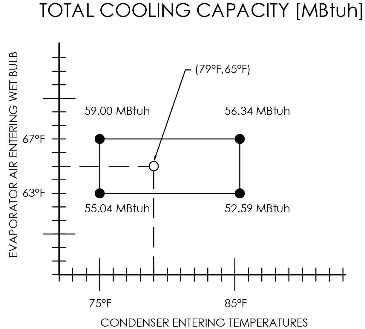
Solution 1: three linear interpolations
- Step 1, at (x,y1): R = 55.04 (85−79)/(85−75) + 52.59 (79−75)/(85−75) = 54.06 MBtuh
- Step 2, at (x,y2): R = 59.00 (85−79)/(85−75) + 56.34 (79−75)/(85−75) = 57.936 MBtuh
- Step 3, at (x,y): R = 54.06 (67−65)/(67−63) + 57.936 (65−63)/(67−63) = 55.998 MBtuh
Solution 2: the single equation
R(x,y) = 55.04(85−79)(67−65)/((85−75)(67−63)) + 52.59(79−75)(67−65)/((85−75)(67−63)) + 59.00(85−79)(65−63)/((85−75)(67−63)) + 56.34(79−75)(65−63)/((85−75)(67−63)) = 55.998 MBtuh
Solution 3: the calculator. Enter the values in the grid above as they appear in the performance table; the center shows 55.998.